In today’s post, I investigate a simple recurrence relation and show how it is possible to describe its behaviour asymptotically at large times. The relation describing how the series evolves at a time n will depend both on its value at the earlier time n/2 and on whether n is even or odd, which, as we will see, introduces a `period doubling’ behaviour in the asymptotics. The proof will involve defining a Dirichlet generating function for the series, showing that it satisfies a functional equation and has a meromorphic extension to the whole complex plane, and then inverting the generating function with Perron’s formula. Cauchy’s residue theorem relates the terms of the asymptotic expansion to the poles of the meromorphic extension of the Dirichlet series. Such an approach is well-known in analytic number theory, originally used by Riemann to give the explicit formula for the prime counting function in terms of the zeros of the Riemann zeta function. However, Dirichlet generating functions can be applied in many other situations to generate asymptotic expansions (see the references for examples). Although I will concentrate on a specific difference equation here, the techniques described are quite general and also apply to many other kinds of series.
This post grew out of an answer I gave to a question by Byron Schmuland at the math.stackexchange website. To motivate the difference equation, let us start by considering the following Markov chain whose state space is the positive integers, as described in the original question by Byron. The chain begins at state 1, and from state n the chain next jumps to a state uniformly selected from 
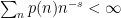
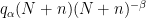
If we define p(n) to be the probability that the chain visits state n, then p(n) goes to zero like c/n for some constant c. In fact,
 |
(1) |
The question asked on math.stackexchange is to give an analytic proof of this fact. It is possible to prove this using a (tricky) probabilistic method and, as explained by Byron and in the other answers to his question, there are quick analytic proofs of conditional convergence. That is, if np(n) does converge to a limit, then it must be the value given in (1). In this post, I use Dirichlet series to not only answer the original question, but also give the entire asymptotic expansion. I am not aware if the results given here are already known although, as noted, it is very similar to asymptotic expansions used in analytic number theory and to the results of Flajolet and Golin mentioned above. The layout of this post is as follows. First, I briefly discuss the recurrence relation satisfied by p and some of the approaches which can be used, as suggested in the original math.stackexchange question. I will then look at the numerical evidence for the behaviour of p, plotting graphs of the first few asymptotic terms. The result of the numerical simulation is used to propose a full asymptotic expansion. Next, the Dirichlet generating function is introduced and a few of its properties, including a functional equation, are proved. The proof of the asymptotic expansion is then given by applying Perron’s formula to invert the generating function. Finally, I end with a few comments about the proof given here.
First, the description of the Markov process above leads to the following recurrence relation for p(n).
 |
(2) |
Alternatively, if we take the difference of p(n+1) and p(n) then most of the terms in the summation above cancel, leading to the difference equation
 |
(3) |
This is just a linear recurrence relation for p, albeit with two complicating factors. First, there is the periodic term 

A probabilistic argument can be given for the limit (1), as given in the answer by `T..’ to the math.stackexchange question. The increase in the logarithm of the position 
![{[0,\log 2]}](https://s0.wp.com/latex.php?latex=%7B%5B0%2C%5Clog+2%5D%7D&bg=ffffff&fg=000000&s=0&c=20201002)


 |
(4) |
where 

Another conditional proof of (1) involves the generating function of p(n)/n,
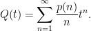 |
(5) |
As the coefficients are bounded by 1/n, the power series converges for all complex 
 |
(6) |
This idea was mentioned by Qiaochu Yuan in his response to the original question, and expanded into a conditional proof of (1) by Byron in the original question. Differentiating again and multiplying by 1-t,
 |
(7) |
Assuming that np(n) converges to a limit c, we can evaluate both sides of (7) to leading order as t goes to 1,
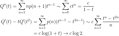
Plugging these limits back into (7) gives
A Numerical Investigation
With the help of a computer, it is easy to simulate p(n) using the recurrence relation (3).
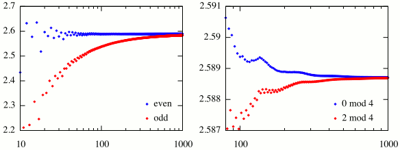
Figure 1 shows two plots of np(n). In the first one, the points are coloured blue for n even and red for n odd (similar to David Speyer’s plot in the math.stackexchange thread linked above). It can be seen that convergence is much faster at even times than at odd times. To see how the series behaves at even times, the second plot only includes those points where n is even, with n a multiple of 4 coloured blue, and n even but not a multiple of 4 coloured red. The simulation suggests that,
- for n odd, np(n) converges to c from below at rate O(1/n).
- for n a multiple of 4, np(n) converges to c from above at rate O(1/n2).
- for n a multiple of 2, but not 4, np(n) converges to c from below at rate O(1/n2).
This suggests the following asymptotic form for p(n)

where 


 |
(8) |
where 


Expanding the left hand side as a Taylor series in 1/n

and comparing coefficients of 

 |
(9) |
This defines 


This defines 

 |
(10) |
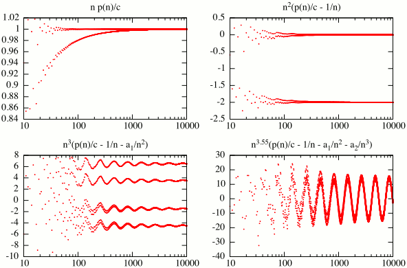
This expansion can be checked by plotting p(n) while successively subtracting out the leading order terms. As can be seen in Figure 2, it converges beautifully to the levels 
However, after 


![{\Re[an^{-r}]}](https://s0.wp.com/latex.php?latex=%7B%5CRe%5Ban%5E%7B-r%7D%5D%7D&bg=ffffff&fg=000000&s=0&c=20201002)


Putting 

 |
(11) |
Looking for solutions with v positive, the first of these equations says that 


The Asymptotic Expansion
The numerical investigation above suggests the following asymptotic expansion for p(n) up to order 
![\displaystyle p(n)=\sum_{\Re[r]+k<\alpha}a_{r,k}(n)n^{-r-k}+O(n^{-\alpha}).](https://s0.wp.com/latex.php?latex=%5Cdisplaystyle++p%28n%29%3D%5Csum_%7B%5CRe%5Br%5D%2Bk%3C%5Calpha%7Da_%7Br%2Ck%7D%28n%29n%5E%7B-r-k%7D%2BO%28n%5E%7B-%5Calpha%7D%29.+&bg=ffffff&fg=000000&s=0&c=20201002) |
(12) |
This sum is taken over complex r satisfying 

The terms 

 |
(13) |
This allows us to calculate 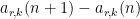


It still remains to calculate the values of 
![\displaystyle p_\alpha(n) \equiv \sum_{\Re[r]+k<\alpha}a_{r,k}(n)n^{-r-k}.](https://s0.wp.com/latex.php?latex=%5Cdisplaystyle++p_%5Calpha%28n%29+%5Cequiv+%5Csum_%7B%5CRe%5Br%5D%2Bk%3C%5Calpha%7Da_%7Br%2Ck%7D%28n%29n%5E%7B-r-k%7D.+&bg=ffffff&fg=000000&s=0&c=20201002) |
(14) |
The fact that the coefficients have been chosen to satisfy (13) means that, if we substitute 
 |
(15) |
The Dirichlet Generating Function
The Dirichlet generating function of the series p(n)/n is

which converges uniformly to an analytic function for the real part of s large. As we know that p is bounded by 1, it will in fact converge for all s with positive real part. It can also be seen that 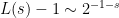

Whereas the standard generating function Q above satisfied a differential equation, the Dirichlet generating function satisfies a functional equation. Multiplying (3) by 

leads to the following functional equation for L,
 |
(16) |
This expresses L(s) in terms of L(s+k) for positive integers k. As L(s) is defined whenever s has positive real part, (16) extends L to all s with real part greater than -1. Inductively applying (16), then, extends L to a meromorphic function on the whole complex plane. The division by 
By a standard result on Dirichlet series with nonnegative coefficients, the fact that L has no poles in the half plane ![{\Re[s]>-1}](https://s0.wp.com/latex.php?latex=%7B%5CRe%5Bs%5D%3E-1%7D&bg=ffffff&fg=000000&s=0&c=20201002)

Noting that 
 |
(17) |
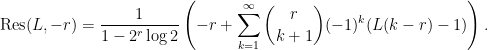
At r=1, all the binomial coefficients on the right hand side are zero, giving the residue
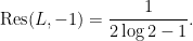 |
(18) |
There does not seem to be a simple expression for the residues at the other poles, although (17) can be used to compute them to whatever accuracy is desired.
We can also write out the Dirichlet generating function for the truncated asymptotic expansion 

This also has a meromorphic expansion to the entire complex plane and the locations and residues of the poles can be determined by the following fact.
- If
is periodic with average value
then
extends to a meromorphic function on the complex plane with a simple pole at s=1 with residue
This result holds whenever a is a Dirichlet character, so f is a Dirichlet L-function and, since all periodic functions 
![{\Re[r]+k<\alpha}](https://s0.wp.com/latex.php?latex=%7B%5CRe%5Br%5D%2Bk%3C%5Calpha%7D&bg=ffffff&fg=000000&s=0&c=20201002)


In particular, from (18), 

![{\Re[r]<\alpha}](https://s0.wp.com/latex.php?latex=%7B%5CRe%5Br%5D%3C%5Calpha%7D&bg=ffffff&fg=000000&s=0&c=20201002)
It is also possible to calculate an approximate functional equation for 
![{\Re[s]\ge\beta}](https://s0.wp.com/latex.php?latex=%7B%5CRe%5Bs%5D%5Cge%5Cbeta%7D&bg=ffffff&fg=000000&s=0&c=20201002)


Summing the remainder term over n converges to an analytic function over 


 |
(19) |
The remainder term R(s) is an analytic function over ![{\Re[s]>-\alpha}](https://s0.wp.com/latex.php?latex=%7B%5CRe%5Bs%5D%3E-%5Calpha%7D&bg=ffffff&fg=000000&s=0&c=20201002)

The above argument for 

Inverting the Dirichlet Series and Proof of the Expansion
The proof of the asymptotic expansion (12) will rely on Perron’s formula to invert the Dirichlet generating function
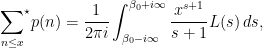
which holds for any 

 |
(20) |
As stated above, this expression is intended in the sense of distributions. That is, if 
 |
(21) |
The term 
![{\beta_0\le\Re[s]\le\beta_1}](https://s0.wp.com/latex.php?latex=%7B%5Cbeta_0%5Cle%5CRe%5Bs%5D%5Cle%5Cbeta_1%7D&bg=ffffff&fg=000000&s=0&c=20201002)

As the Dirichlet generating function L is polynomially bounded on each half-plane for large s, it follows that the integrand on the right hand side of (21) goes to zero faster than polynomially in 1/s, and the integral in (20) is well defined in the sense of distributions on any line ![{\Re[s]=\beta_0}](https://s0.wp.com/latex.php?latex=%7B%5CRe%5Bs%5D%3D%5Cbeta_0%7D&bg=ffffff&fg=000000&s=0&c=20201002)
The idea is to move the line of integration in (20) to the left, using Cauchy’s residue theorem to pick up terms from the poles of L,
![\displaystyle \phi(x)=\sum_{\Re[r]+k+\beta<0}{\rm Res}(L,-r-k)x^{-r-k}+\frac{1}{2\pi i}\int_{\beta-i\infty}^{\beta+i\infty}x^sL(s)\,ds](https://s0.wp.com/latex.php?latex=%5Cdisplaystyle++%5Cphi%28x%29%3D%5Csum_%7B%5CRe%5Br%5D%2Bk%2B%5Cbeta%3C0%7D%7B%5Crm+Res%7D%28L%2C-r-k%29x%5E%7B-r-k%7D%2B%5Cfrac%7B1%7D%7B2%5Cpi+i%7D%5Cint_%7B%5Cbeta-i%5Cinfty%7D%5E%7B%5Cbeta%2Bi%5Cinfty%7Dx%5EsL%28s%29%5C%2Cds+&bg=ffffff&fg=000000&s=0&c=20201002) |
(22) |
for any real 
![{\Re[s]=\beta}](https://s0.wp.com/latex.php?latex=%7B%5CRe%5Bs%5D%3D%5Cbeta%7D&bg=ffffff&fg=000000&s=0&c=20201002)


![{[\beta,\beta_0]\times[-u,u]}](https://s0.wp.com/latex.php?latex=%7B%5B%5Cbeta%2C%5Cbeta_0%5D%5Ctimes%5B-u%2Cu%5D%7D&bg=ffffff&fg=000000&s=0&c=20201002)

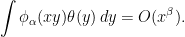
Equation (22) holds in the sense of distributions. We can convolve both sides by an infinitely differentiable function 
![\displaystyle \setlength\arraycolsep{2pt} \begin{array}{rl} \displaystyle\int\phi(xy)\theta(y)\,dy=&\displaystyle\sum_{n=1}^\infty p(n)\theta(n/x)/x\smallskip\\ =&\displaystyle\sum_{\Re[r]+k+\beta<0}{\rm Res}(L,-r-k)x^{-r-k}\int y^{-r-k}\theta(y)\,dy\smallskip\\ &\displaystyle+\frac{1}{2\pi i}\int_{\beta-i\infty}^{\beta+i\infty} x^s\int y^s\theta(y)\,dy L(s)\,ds \end{array}](https://s0.wp.com/latex.php?latex=%5Cdisplaystyle++%5Csetlength%5Carraycolsep%7B2pt%7D+%5Cbegin%7Barray%7D%7Brl%7D+%5Cdisplaystyle%5Cint%5Cphi%28xy%29%5Ctheta%28y%29%5C%2Cdy%3D%26%5Cdisplaystyle%5Csum_%7Bn%3D1%7D%5E%5Cinfty+p%28n%29%5Ctheta%28n%2Fx%29%2Fx%5Csmallskip%5C%5C+%3D%26%5Cdisplaystyle%5Csum_%7B%5CRe%5Br%5D%2Bk%2B%5Cbeta%3C0%7D%7B%5Crm+Res%7D%28L%2C-r-k%29x%5E%7B-r-k%7D%5Cint+y%5E%7B-r-k%7D%5Ctheta%28y%29%5C%2Cdy%5Csmallskip%5C%5C+%26%5Cdisplaystyle%2B%5Cfrac%7B1%7D%7B2%5Cpi+i%7D%5Cint_%7B%5Cbeta-i%5Cinfty%7D%5E%7B%5Cbeta%2Bi%5Cinfty%7D+x%5Es%5Cint+y%5Es%5Ctheta%28y%29%5C%2Cdy+L%28s%29%5C%2Cds+%5Cend%7Barray%7D+&bg=ffffff&fg=000000&s=0&c=20201002)
The left hand side of this expression is a weighted sum of p(n) for n in a region near x. The integrand of the contour integral on the right hand side consists of a term going to zero faster than polynomially in 1/s multiplied by a term of size 
![\displaystyle \int\phi(xy)\theta(y)\,dy = \sum_{\Re[r]+k+\beta<0}{\rm Res}(L,-r-k)x^{-r-k}\int y^{-r-k}\theta(y)\,dy + O(x^\beta).](https://s0.wp.com/latex.php?latex=%5Cdisplaystyle++%5Cint%5Cphi%28xy%29%5Ctheta%28y%29%5C%2Cdy+%3D+%5Csum_%7B%5CRe%5Br%5D%2Bk%2B%5Cbeta%3C0%7D%7B%5Crm+Res%7D%28L%2C-r-k%29x%5E%7B-r-k%7D%5Cint+y%5E%7B-r-k%7D%5Ctheta%28y%29%5C%2Cdy+%2B+O%28x%5E%5Cbeta%29.+&bg=ffffff&fg=000000&s=0&c=20201002) |
(23) |
This expression is very close to the asymptotic expansion (12). It differs by replacing p(n) on the left hand side by a `smoothed’ version of p. Also, although the right hand side does have a term corresponding to each of the terms 

There does not seem to be any way that periodic behaviour of the coefficients can come out of a direct application of Cauchy’s residue theorem in this way. So, instead, we can look at the difference 


 |
(24) |
This holds for any 

 |
(25) |
Here, I am using 


![{[1,1+\epsilon]}](https://s0.wp.com/latex.php?latex=%7B%5B1%2C1%2B%5Cepsilon%5D%7D&bg=ffffff&fg=000000&s=0&c=20201002)

However, K can be chosen arbitrarily large, so this contradicts the bound (24). It follows that 


for any 


This is exactly the asymptotic expansion proposed in (12).
Notes
It is useful to note why the Dirichlet generating function works in this proof, whereas the standard power series generating function defined in (5) does not. There is a similar inversion formula to (20) for Q, using Cauchy’s integral formula.

where C is any closed curve in the unit disc winding once anticlockwise about the origin. If Q extended to a meromorphic function on some neighbourhood of the unit disc, then we could move the curve C outwards so that it lies on a circle of radius 

However, we know that the series p(n) is not like this. It has asymptotics decaying at rate
From a slightly different point of view, the generating function Q did not satisfy a functional equation which could directly give us a meromorphic expansion. Instead, it satisfied a differential equation (6). The reason for this is that the 1/n terms on the right hand side of (3) lead to a differential term in the expression for the generating function. On the other hand, multiplying a series by 1/n only causes its Dirichlet generated function to be translated by 1, so we obtain a functional equation (16) capable of generating a meromorphic extension to the whole complex plane.
It was noted above that, because of the p(n/2) term in the recurrence relation (3), it should be no surprise that the asymptotic expansion includes infinitely many independent terms. We can also see how this infinite set of terms arises, by looking at the functional equation (16) for L. The p(n/2) term leads to the 
The proof given above is, largely, quite standard and very similar to other well known proofs of asymptotic expansions. This involves the following steps,
- Define a (Dirichlet) generating function.
- Establish a functional equation.
- Using the functional equation, prove the existence of a meromorphic extension.
- Use Perron’s formula to express the original series as a contour integral.
- Move the line of integration to the left, using Cauchy’s residue theorem to pick up asymptotic terms from the poles of the generating function.
There are, not surprisingly, further technicalities. It is necessary to use a bound on the growth of the generating function in order to bound the contour integrals. Above, I made use of the fact that L(s) is polynomially bounded on each half-plane.
However, there was one further complicating issue in the proof above, requiring a bit of back-and-forth between the Dirichlet series and the approximate recurrence relation (15). This is because, as was noted, there is no way that Cauchy’s residue theorem would give the correct periodic coefficients in the expansion. Instead, we obtained a formula for a smoothed version of the version of the series which averaged out the periodic terms. Applying this to the remainder term 

for complex roots of unity 


References
- Michael Drmota and Wojciech Szpankowski. A General Discrete Divide and Conquer Recurrence and Its Applications. Preprint, 2010. Available from Michael Drmota’s homepage.
- Philippe Flajolet and Mordecai Golin. Exact asymptotics of divide-and-conquer recurrences. Lecture notes in Computer Science, 1993, Volume 700, 137-149.
- Fillippe Flajolet and Robert Sedgewick. Analytic Combinatorics. Cambridge University Press, 2009.
- Hsien-Kuei Hwang. Asymptotic expansions of the mergesort recurrences. Acta Informatica, 1998, Volume 35, Number 11, 911-919.

George,
Let me be the first to thank you for the incredible amount of work that you put into this problem. I have been thinking about this problem for a long time, and am very grateful to see the “correct” approach to such recurrences. I look forward to reading your explanation in detail and delving into the references.
No problem. It was a very interesting question, and was fun to work out. This kind of problem, and the solution, are new to me, and I don’t know if it has been studied before. The recurrences studied in the references have some similarity to this one, and Dirichlet generating functions are used. The asymptotics are rather different to the recurrence studied here though, and don’t have the periodic coefficients. If I come across any better references, I’ll add them to the list.