The Stochastic Integral

George Lowther Stochastic Calculus Notes, Stochastic Integration 3 January 107 April 21

Having covered the basics of continuous-time processes and filtrations in the previous posts, I now move on to stochastic integration. In standard calculus and ordinary differential equations, a central object of study is the derivative ${df/dt}$ of a function ${f(t)}$ . This does, however, require restricting attention to differentiable functions. By integrating, it is possible to generalize to bounded variation functions. If ${f}$ is such a function and ${g}$ is continuous, then the Riemann-Stieltjes integral ${\int_0^tg\,df}$ is well defined. The Lebesgue-Stieltjes integral further generalizes this to measurable integrands.

However, the kinds of processes studied in stochastic calculus are much less well behaved. For example, with probability one, the sample paths of standard Brownian motion are nowhere differentiable. Furthermore, they have infinite variation over bounded time intervals. Consequently, if ${X}$ is such a process, then the integral ${\int_0^t\xi\,dX}$ is not defined using standard methods.

Stochastic integration with respect to standard Brownian motion was developed by Kiyoshi Ito. This required restricting the class of possible integrands to be adapted processes, and the integral can then be constructed using the Ito isometry. This method was later extended to more general square integrable martingales and, then, to the class of semimartingales. It can then be shown that, as with Lebesgue integration, a version of the bounded and dominated convergence theorems are satisfied.

In these notes, a more direct approach is taken. The idea is that we simply define the stochastic integral such that the required elementary properties are satisfied. That is, it should agree with the explicit expressions for certain simple integrands, and should satisfy the bounded and dominated convergence theorems. Much of the theory of stochastic calculus follows directly from these properties, and detailed constructions of the integral are not required for many practical applications. Before moving on to the definition, note that, whereas the value of a standard Lebesgue integral is just a real number, stochastic integrals take values in the space of random variables. It is therefore possible to weaken some of the properties required of such integrals. First, any identity is only required to be satisfied almost surely. That is, on a set of probability one. Second, the notion of convergence of a sequence of real numbers can be replaced by the much weaker idea of convergence in probability.

We work with respect to a complete filtered probability space ${(\Omega,\mathcal{F},\{\mathcal{F}_t\}_{t\ge 0},{\mathbb P})}$ . Then, the space of random variables is denoted by ${L^0(\Omega,\mathcal{F},{\mathbb P})}$ , or simply ${L^0}$ . This is the space of measurable functions ${\Omega\rightarrow{\mathbb R}}$ or, more precisely, the equivalence classes of such functions up to equality on a set of probability one.

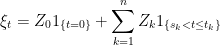
Recall that an elementary predictable process ${\xi}$ is of the form

$\displaystyle \xi_t=Z_01_{\{t=0\}}+\sum_{k=1}^nZ_k1_{\{s_k<t\le t_k\}}$

for ${n\ge 0}$ , times ${s_k<t_k}$ , ${\mathcal{F}_0}$ -measurable random variable ${Z_0}$ and ${\mathcal{F}_{s_k}}$ -measurable random variables ${Z_k}$ . The stochastic integral of this with respect to a process ${X}$ is

$\displaystyle \int_0^t\xi\,dX = \sum_{k=1}^nZ_k\left(X_{t_k\wedge t}-X_{s_k\wedge t}\right).$

(1)

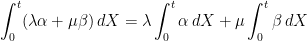
Integration is a linear function of the integrand, so that

$\displaystyle \int_0^t(\lambda\alpha+\mu\beta)\,dX = \lambda\int_0^t\alpha\,dX + \mu\int_0^t\beta\,dX$

(2)

for real numbers ${\lambda,\mu}$ and predictable processes ${\alpha,\beta}$ .

Also, the stochastic integral should satisfy bounded convergence in probability. That is, if ${\xi^n}$ is a sequence of predictable processes converging to a limit ${\xi}$ , and is uniformly bounded ${\vert\xi^n\vert\le K}$ for some constant ${K>0}$ , then the integrals converge,

$\displaystyle \int_0^t\xi^n\,dX\rightarrow\int_0^t\xi\,dX\ \ \text{(in probability)}.$

(3)

These properties are enough to define stochastic integration for bounded and predictable integrands. The notation ${{\rm b}\mathcal{P}}$ is used to denote the bounded predictable processes.

Definition 1 Let ${X}$ be a process. The stochastic integral up to time ${t\ge 0}$ with respect to ${X}$ , if it exists, is a map

$\displaystyle {\rm b}\mathcal{P}\rightarrow L^0,\ \xi\mapsto\int_0^t\xi\,dX$

which

agrees with the explicit expression (1) for bounded elementary integrands ${\xi}$ .

satisfies bounded convergence in probability (3).

Proving the existence of the stochastic integral for an arbitrary integrator ${X}$ is, in general, quite a difficult problem. However, uniqueness is a simple consequence of the monotone class theorem. Also, note that the requirement that the integral is a linear function of the integrand was not mentioned in the definition above. However, this property is again a simple consequence of the monotone class theorem.

Lemma 2 Let ${X}$ be a stochastic process. If the stochastic integral up to time ${t\ge 0}$ as given by Definition 1 exists, then it is uniquely defined. Furthermore, linearity in the integrand (2) is satisfied.

Proof: Suppose that there were two versions of the integral, both satisfying the required properties. Denoting them by ${I(\xi)}$ and ${J(\xi)}$ respectively, let ${V}$ be the set of all bounded predictable processes satisfying ${I(\xi)=J(\xi)}$ . From the definition above, this includes all bounded elementary integrands and is closed under bounded convergence. However, the elementary predictable processes generate the predictable sigma-algebra. So, by the monotone class theorem, ${V}$ contains all bounded predictable processes, and ${I=J}$ .

Linearity follows in a similar way. For elementary integrands, it follows from equation (3). More generally, fix real ${\lambda,\mu}$ and bounded elementary ${\alpha}$ . Then, let ${V}$ consist of the set of bounded predictable processes ${\beta}$ such that (2) is satisfied. Again, this includes the elementary processes and is closed under bounded convergence. So, (2) is satisfied for all elementary ${\alpha}$ and bounded predictable ${\beta}$ .

Finally, fix a bounded predictable process ${\beta}$ and let ${V}$ be the set of all bounded predictable processes ${\alpha}$ such that (2) is satisfied. As proven above, this contains all elementary processes. Also, it is closed under bounded convergence, so (2) is satisfied for all ${\alpha,\beta\in{\rm b}\mathcal{P}}$ . ⬜

Any process with respect to which the stochastic integral is well defined must necessarily satisfy certain basic properties.

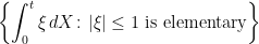
Lemma 3 Let ${X}$ be an adapted stochastic process such that, for each ${t\ge 0}$ , the stochastic integral ${\int_0^t\xi\,dX}$ given by Definition 1 exists. Then,

${X}$ is right-continuous in probability.

The set

$\displaystyle \left\{\int_0^t\xi\,dX\colon\vert\xi\vert\le 1\text{ is elementary}\right\}$ (4)

is bounded in probability, for each ${t\ge 0}$ .

${X}$ has a cadlag verson.

Proof: If ${t_n\downarrow t}$ is a sequence of times, then bounded convergence gives

$\displaystyle X_{t_n}-X_t=\int_0^{t_1}1_{\{t<s\le t_n\}}\,dX_s\rightarrow 0$

in probability as ${n\rightarrow\infty}$ . So, ${X}$ is right-continuous in probability.

Next, we can show that the set of integrals ${\int_0^t\xi\,dX}$ for predictable integrands ${\vert\xi\vert\le1}$ is bounded in probability, for each fixed time ${t\ge0}$ . In particular, by restricting to elementary integrands, this will imply that (4) is bounded in probability.

Arguing by contradiction, suppose that this is not the case. By definition, this means that there is an ${\epsilon>0}$ and a sequence of predictable processes ${\vert\xi^n\vert\le 1}$ such that ${{\mathbb P}(\vert\int_0^t\xi^n\,dX\vert>n)>\epsilon}$ for all n. However, this contradicts bounded convergence in probability,

$\displaystyle {\mathbb P}\left(\left\vert\int_0^t\xi^n\,dX\right\vert>n\right)={\mathbb P}\left(\left\vert\int_0^tn^{-1}\xi^n\,dX\right\vert>1\right)\rightarrow 0$

as ${n\rightarrow\infty}$ . Hence, the set given by (4) must indeed be bounded in probability.

Finally, using a result from an earlier post, the existence of cadlag versions follows from the first two properties and the condition that the process is adapted. ⬜

The first two conditions above are not only necessary for the existence of the stochastic integral, they are also sufficient. That fact is not needed here though, and the existence of the integral given these conditions will be shown in a later post. Adapted processes with respect to which stochastic integration is well defined are known as semimartingales. By the result above, there is no loss of generality in only considering cadlag processes.

Definition 4 A semimartingale ${X}$ is a cadlag adapted process such that, for each ${t\ge 0}$ , the stochastic integral given by Definition 1 exists.

Simple examples of semimartingales include the cadlag adapted processes of finite variation over all bounded time intervals. Then, the stochastic integral of Definition 1 coincides with the Lebesgue-Stieltjes integral. More interesting examples include Brownian motion and, as we shall see later, all local martingales.

As mentioned above, the stochastic integral was originally constructed with respect to Brownian motion and, then, similar techniques were applied to arbitrary martingales. This led, historically, to the definition of a semimartingale as a process which can be decomposed into a sum of a finite variation process and a local martingale. That such processes are in fact equivalent to the definition above is a consequence of the Bichteler-Dellacherie theorem which will be covered later in these notes.

Published by George Lowther

View all posts by George Lowther

Published 3 January 107 April 21

37 thoughts on “The Stochastic Integral”

idontgetoutmuch says:

10 July 11 at 8:24 AM

In Chapter 2, Protter defines a process ${X}$ to be a total semimartingale if ${X}$ is càdlàg, adapted, and ${I_X : {\bf S}_u \longrightarrow {\bf L}^0}$ is continuous where ${{\bf S}}$ is the collection of simple predictable processes topologized by uniform convergence in ${(t,\omega)}$ and ${{\bf L}^0}$ is the space of finite-valued random variables topologized by convergence in probability.

He further defines a semimartingale to be a total semimartingale ${X}$ stopped at a fixed time ${t \in [0,\infty)}$ denoted ${X^t}$ .

Theorem 8, Chapter 2 states:

Each ${L^2}$ martingale with càdlàg paths is a semimartingale.

Corollary 1 to this theorem states:

Each càdlàg, locally square integrable local martingale is a semimartingale.

Corollary 2 to this theorem states:

A local martingale with with continuous paths is a semimartingale.

And as proof states:

Apply Corollary 1 together with Theorem 51 in Chapter 1.

Now Theorem 51 states:

Let ${X}$ be a local martingale such that ${\mathop{\mathbb E} X^*_t < \infty}$ for every ${t \geq 0}$ . Then ${X}$ is a martingale. If ${\mathop{\mathbb E} X^* < \infty}$ , then X is a uniformly integrable martingale.

In order to apply Corollary 1 we need to show that the local martingale we are given is locally square integrable. But how does Theorem 51 help with this? The premise for second part of Theorem 51 does not even hold, for example, take ${X}$ to be Brownian Motion.

Reply
1. George Lowther says:
  
  18 July 11 at 11:21 PM
  
  Hi.
  
  [Aside: Protter’s definition of a semimartingale is (seemingly) weaker than the one I gave in this post, as I required the existence of a stochastic integral as part of the definition. The equivalence between the two definitions is proven in the post Existence of the Stochastic Integral and restated as part of the Bichteler-Dellacherie Theorem.]
  
  On to your question. You just want to show that the continuous local martingale X is locally a square integrable martingale. This uses continuity. Let $\tau_n$ be the first time t at which |X_t| ≥ n. Continuity tells you that $X^{\tau_n}$ is bounded by n and Theorem 51 tells that it is a martingale. Actually, Theorem 51 is not really needed because once you know that $X^{\tau_n}$ are locally square integrable martingales, the same is true of X. Theorem 51 does shorten the argument slightly though. Hope that helps.
  
  Reply
  1. Anonymous says:
    
    27 July 11 at 8:17 AM
    
    That does thanks very much. Good notes by the way.
    
    Reply
Abdeldjebbar says:

25 October 11 at 2:31 PM

Can I have all these notions in the same file because it is very interest for me.

[George: I edited your email address out. Are you sure you wanted it here for everyone to see? I can add it back if you want.]

Reply
1. George Lowther says:
  
  27 October 11 at 1:02 PM
  
  Hi.
  
  I’m glad you find these interesting. I will join them together into a single file at some point, and post them on this site. Probably after I have completed the next few posts so that the ‘general theory of semimartingales’ section is complete.
  
  I can’t just join them together immediately, as it will need some work to link them together making sure that subheadings, links, etc are working properly. So, like I say, it will probably be after I have completed the current section.
  
  Reply
Alex says:

1 March 12 at 12:56 PM

Dear George,
I keep noticing in the literature on stochastic processes that the assumption about completeness of the probability space is made at the very beginning. But the authors don’t point out where the assumption is actually used. I was very glad to see that you made the same assumption and I can ask you about it. Why is it important and in what cases it is not required?
Thank you.
Alex.

Reply
1. George Lowther says:
  
  4 March 12 at 3:57 PM
  
  There’s a few places where completeness of the filtration is used. It is not really necessary, but it helps simplify things.
  
  i) To ensure that processes have adapted cadlag modifications. In particular – martingales, sub(super)martingales, Feller processes, processes for which the stochastic integral is well defined (see Lemma 3 above). You don’t really need completeness for this, just requiring $\mathcal{F}_0$ to contain all zero probability sets in $\mathcal{F}_\infty$ is enough. This did come up in an earlier comment to the post on cadlag modifications.
  ii) To ensure that hitting times are stopping times (debut theorem). Completeness is not really needed because usually it is enough to find a stopping time which is almost surely equal to the hitting time (again, this has come up in a previous comment).
  iii) To ensure that stochastic integrals have a cadlag modification. Even if X is a semimartingale and, hence, is cadlag by definition, it does not follow that stochastic integrals $\int\xi\,dX$ have adapted cadlag modifications. Using dominated convergence, you can show that it has a modification which is almost surely cadlag. This is probably all that you need, although it helps to as least assume that $\mathcal{F}_0$ contains the zero probability sets of $\mathcal{F}_\infty$ , so that you can use cadlag adapted versions of the integral.
  
  Reply
  1. Anonymous says:
    
    5 May 12 at 7:42 PM
    
    Dear George,
    I have a question on that completeness issue. You say that instead of completeness of filtrations we can add zero probability sets from F_oo to F_t. Does F_oo have to be complete?
    Thank you.
    Alex.
    
    Reply
    1. George Lowther says:
      
      6 May 12 at 1:20 AM
      
      If you want the debut theorem to hold then, yes, you do need $\mathcal{F}_\infty$ to be complete or – at least – universally complete. For most other results, you do not need $\mathcal{F}_\infty$ to be complete.
    2. Anonymous says:
      
      7 May 12 at 12:53 PM
      
      But the completeness seems to be a requirement as pointed out by some authors. For example, in Krylov “Introduction to the theory of diffusion procesess”, p.94. In the remark he says that the completeness of the filtration is requred for the stochastic integral (wrt a Brownian motion) to be adapted. The reason is the following.
      We want the integral wrt a BM to be continuous and adapted. When defining the stochastic integral, it is possible to find simple processes such that their integrals are continuous and converge uniformly with probability 1, and thus, the continuity is preserved almost surely. Since the convergence is only in almost sure sense, the limit does not have to be adapted unless the filtration is complete.
      SImilar construction in Liptser, Shiryaev “Statistics of random processes”, V.2, p.102 also requires the filtration to be augmented by all zero sets from the original sigma-algebra which is assumed to be complete.
      Could you please explain these deferences in construction of stochastic integrals (for example, wrt Brownian motion)? For what cases we have to require the filtration (and or the original probability space) to be complete?
    3. George Lowther says:
      
      7 May 12 at 7:45 PM
      
      When defining the stochastic integral, it is possible to find simple processes such that their integrals are continuous and converge uniformly with probability 1, and thus, the continuity is preserved almost surely. Since the convergence is only in almost sure sense, the limit does not have to be adapted unless the filtration is complete.
      
      Note quite. If a sequence of (simple) integrals $\int\xi^n\,dX$ converges uniformly with probability 1, to a limit $\int\xi\,dX$ , then there exists a set $A\in\mathcal{F}_\infty$ with probability 1 such that convergence is uniform on A. We know that A can be taken to be in $\mathcal{F}_\infty$ because each of the simple integrals is $\mathcal{F}_\infty$ -measurable. Then, you can take $\int\xi\,dX=\lim_{n\to\infty}1_A\int\xi^n\,dX$ which converges uniformly and, hence, is continuous. So, we need to know that A is in $\mathcal{F}_t$ for all t, which is guaranteed by the requirement that all zero probability sets in $\mathcal{F}_\infty$ are in $\mathcal{F}_0$ . Completeness is a stronger condition than is necessary.
  2. Anonymous says:
    
    9 May 12 at 1:10 PM
    
    Dear Goerge, thank you very much for spending your time on this discussion. However, you say
    
    “Then, you can take $\int\xi\,dX=\lim_{n \to \infty} 1_{A} \int\xi^n\,dX$ which converges uniformly and, hence, is continuous.”
    
    Here, you define the integral to be 0, outside the set A which actually yields \omega-wise continuity (not P-a.s. continuity). This way of defining the integral is fine. However, if we do not make this assumption and the only thing that we know is that it is possible to find a sequence of simple processes (continuous and adapted) that converge uniformly P-a.s. is it still enough to add all zero sets from F_oo (not complete) to F_t to claim that the limit process is adapted?
    
    Reply
    1. George Lowther says:
      
      9 May 12 at 8:51 PM
      
      I’m not exactly sure what you are asking now. So long as you add all zero sets from $\mathcal{F}_\infty$ to $\mathcal{F}_0$ then it is possible to construct a stochastic integral which is both adapted and satisfies all the usual pathwise properties (cadlag, etc). If, on the other hand, you have already constructed the integral in such a way that the usual properties are satisfied (which are only specified in an almost sure sense) then, no, you can’t guarantee that it is adapted unless you complete the filtration. In fact, just looking at real valued random variables (so, no processes and no integration), if a sequence of random variables X_n almost-surely converges to a limit X then it is only guaranteed that X is measurable on the set where this convergence holds. So, you can only conclude that X is measurable if the probability space is complete.
  3. Anonymous says:
    
    10 May 12 at 1:56 PM
    
    Yes, now I see that this requirement depends on the way the stochastic integral is constructed. In the two mentioned books this assumption is used. However, it seems like the integral can be constructed without this assumption. Thank you very much again for explaining this issue.
    
    Reply
Wolfgang says:

20 April 12 at 11:07 PM

I have a problem with the proof of linearity in the integrand in Lemma 2. You check that V contains the elementary processes and is closed under bounded convergence. But the monoton class theorem requires V to be a vector space too. Is it necessary to include linearity in Definition 1?

Reply
1. George Lowther says:
  
  22 April 12 at 2:17 AM
  
  Hi. No, it is not necessary to include linearity. Obviously, we do want linearity and it might be worthwhile including it in the definition to emphasize this fact, but it is not necessary.
  
  Also, I don’t think it is quite true that the monotone class theorem requires V to be a vector space. Most statements do require this, but there are several slightly different ways of stating the monotone class theorem, which start from different premises. I have been intending to include a post on the monotone class theorem for some time, as I don’t know any really good online resource for it to link to.
  
  You should be able to prove the following though. Let (X,𝒜) be a measurable space, V, W sets of bounded functions f:X->R such that.
  (i) W is contained in V.
  (ii) W is closed under taking linear combinations.
  (iii) There exists a pi-system 𝒮 generating the sigma algebra 𝒜 such that the indicator function 1_S is in W for all S ∈ 𝒮
  (iv) V is closed under taking limits of uniformly bounded sequences.
  Then, V contains all the 𝒜 measurable and bounded functions from X to R.
  
  Consider letting V₁ be the set of all functions f in V such that af+g is in V for all real a and g in W.
  Let V₂ be the set of all functions f in V₁ such that af+g is in V₁ for all real a and g in V₁.
  
  Show that V₂ satisfies the properties above ascribed to V, and is also closed under taking linear combinations. You can now apply the monotone class theorem to V₂ to conclude that it (and hence, also V) contains all bounded and measurable functions f:X->R.
  
  In the context of Lemma 2, W would be the space of bounded elementary integrands and V would be the set of bounded predictable processes for which the integral is uniquely defined.
  
  Reply
  1. Wolfgang says:
    
    22 April 12 at 7:42 PM
    
    Dear George,
    
    thanks for your quick reply. This completely solves my problem with the proof of linearity in Lemma 2.
    
    Reply
  2. toultoutim says:
    
    24 April 12 at 3:05 PM
    
    Hi George,
    
    The idea to write a post about Monotone Class Theorem … and all its functional cousins is a very good idea. Personally, I find painfull textbook’s that only give as a proof for a theorem a sentence such as “by a Monotone Class Argument… the result follows they should at least define the collection of sets (or functions), that are the $\lambda$ -systems and or $\pi$ -systems (or functional equivalents) to plug in the MCT. Anyway a “userguide for MCT” would be a valuable item of your blog.
    
    Best regards.
    
    Reply
    1. George Lowther says:
      
      3 May 12 at 1:49 AM
      
      toultoultim: I’ll work on this – probably won’t be the very next entry, more likely in a few posts time.
    2. George Lowther says:
      
      28 October 19 at 4:50 PM
      
      May be a bit late for toultoutim, but here is the post https://almostsure.wordpress.com/2019/10/27/the-functional-monotone-class-theorem
josh says:

22 September 12 at 1:19 AM

Dear George,
Thanks a lot for your great blog. I learn a lot from it.
Here is my question. Sorry if it is stupid. You write above:
“Also, the stochastic integral should satisfy bounded convergence in probability. That is, if is a sequence of predictable processes converging to a limit …”
You have probably explained somewhere in what sense the sequence of predictable processes does converge, but I am unable to find where. Or is it obvious ? Is it UCP convergence or almost sure uniform convergence on compact sets ?
Thanks and regards

Reply
Alex says:

27 February 14 at 4:53 PM

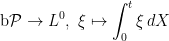
Dear George,
Thank you for your notes. However, I have a question. Let $X_t$ be a continuous martingale. What should be the requirements for the process b in the stochastic integral
$\int_0^t dX_s/b(X_s)$
For some reason in Liptser, Shiryaev (2001) on page 200, the requirement is b^2 >= c > 0. Is it really necessary for the integrand to be bounded?
Thank you.
Best,
Alex.

Reply
1. George Lowther says:
  
  26 October 19 at 4:11 AM
  
  You just need $b(X_t)^{-1}$ to be X-integrable. For a continuous martingale, this is equivalent to $\int_0^t b(X_s)^{-2}d[X]_s$ to be almost-surely finite at each positive time t. Clearly, 1/b being bounded is sufficient, but is not necessary. See my post on continuous local martingales at https://almostsure.wordpress.com/2010/04/01/continuous-local-martingales.
  
  Reply
Anonymous says:

13 December 15 at 1:18 AM

great $x$

Reply
ivan890101 says:

11 July 18 at 2:52 AM

Dear George,

thanks for your notes. They have helped me a lot to understand some abstract parts of Protter’s book.

Reply
Carlo Cabrera says:

28 September 19 at 5:36 AM

Your link to the monotone class theorem is broken. The correct URL is .

Reply
1. Carlo Cabrera says:
  
  28 September 19 at 5:37 AM
  
  Ok, I formatted my previous comment wrong. This is the URL: https://planetmath.org/functionalmonotoneclasstheorem
  
  Reply
  1. George Lowther says:
    
    30 September 19 at 10:57 PM
    
    Thanks, I fixed it.
    
    Reply
Zhouyi says:

20 October 19 at 8:20 PM

In your condition (3), which mode of convergence of $\xi_n$ to $\xi$ are you using? I guess it is a.s. convergence. In the proof of Lemma 3, the integrand $1_{t<s\leq t_n}$ does not converge uniformly to 0 nor in ucp.

Reply
1. George Lowther says:
  
  29 October 19 at 2:26 PM
  
  It is pointwise convergence. $\xi^n_t(\omega)\to\xi_t(\omega)$ for each $\omega\in\Omega$ and $t\in\mathbb R^+$ . Or, you can use almost all $\omega\in\Omega$ , it makes no difference.
  
  Reply
Ilya Zakharevich says:

27 March 21 at 8:44 AM

“Simple examples of semimartingales include the cadlag adapted processes which of finite variation over all bounded time intervals.”

“which” seems to be extraneous… [GL: Fixed, thanks!]

Reply
H W says:

9 June 21 at 3:39 AM

I have questions about: [Between Eq. (2) and (3)], you have stated that, “…if {\xi^n} is a sequence of predictable processes converging to a limit {\xi}…”….(0) What would be a/the metric? (1) converge in which sense? (2) Do all x_i’s have to have jumps at the same times? (3) I may have misunderstood…the jump-times ti_i are deterministic; what would happen if they were stopping times…now, I have the same doubt as in (2)…would the “composition of random functions” type argument work or there is more to it?

Reply
1. George Lowther says:
  
  25 February 22 at 2:00 PM
  
  – Just pointwise convergence. $\xi^n_t(\omega)$ converges for each $t\in\mathbb R^+$ and $\omega\in\Omega$ .
  – They do not have to jump at the same time, this is not required for pointwise convergence.
  – You can generalize to stopping times without much trouble, although then you do need a good version of X (eg, right-continuous) from the start.
  – I am not sure what you mean by “composition of random functions” type argument.
  
  Reply
  1. H W says:
    
    31 May 22 at 2:01 PM
    
    Sorry my my very late reply. By “composition” I had meant function of a function.
    
    Reply
RozaTh says:

14 August 22 at 7:32 PM

Hi, there is a possible typo in the proof of Lemma 2, second paragraph: “Linearity follows in a similar way. For elementary integrands, it follows from equation (3).” I think it should be “it follows from equation (1).”

Reply
Dylan P. says:

13 October 22 at 12:32 PM

Dear George,

I have a more generic question here about your construction of the stochastic integral in this blog. The whole approach seems to be restricted to one-dimensional semi-martingales, and thus a priori does not cover vector stochastic integration, since it cannot simply be defined directly from the one-dimensional case.

I haven’t tried to check if there were places where you crucially needed the one-dimension assumption, but I was wondering if this was done for simplicity, and you expect that everything can be extended mutatis mutandis, or if there may be some parts where you already suspect the construction would fail.

Thanks a lot!

Reply
1. Anonymous says:
  
  19 March 24 at 7:08 AM
  
  Dear George,
  
  Just wanted to check if you had seen this post, since it’s been a moment :).
  
  Thanks!
  
  Reply

	Anonymous on About
	Anonymous on About
	Anonymous on The Stochastic Integral
	Anonymous on Bessel Processes
	Anonymous on Bessel Processes
	Stat Prof on Pathwise Regularity of Optiona…
	Yang Chu on Spitzer’s Formula
	Anonymous on About
	Anonymous on Continuous Processes with Inde…
	Anonymous on Continuous Processes with Inde…

Related

Published by George Lowther

37 thoughts on “The Stochastic Integral”

Leave a comment Cancel reply