Failure of the Martingale Property

In this post, I give an example of a class of processes which can be expressed as integrals with respect to Brownian motion, but are not themselves martingales. As stochastic integration preserves the local martingale property, such processes are guaranteed to be at least local martingales. However, this is not enough to conclude that they are proper martingales. Whereas constructing examples of local martingales which are not martingales is a relatively straightforward exercise, such examples are often slightly contrived and the martingale property fails for obvious reasons (e.g., double-loss betting strategies). The aim here is to show that the martingale property can fail for very simple stochastic differential equations which are likely to be met in practice, and it is not always obvious when this situation arises.

Consider the following stochastic differential equation

$\displaystyle \setlength\arraycolsep{2pt} \begin{array}{rl} &\displaystyle dX = aX^c\,dB +b X dt,\smallskip\\ &\displaystyle X_0=x, \end{array}$

(1)

for a nonnegative process X. Here, B is a Brownian motion and a,b,c,x are positive constants. This a common SDE appearing, for example, in the constant elasticity of variance model for option pricing. Now consider the following question: what is the expected value of X at time t?

The obvious answer seems to be that ${{\mathbb E}[X_t]=xe^{bt}}$ , based on the idea that X has growth rate b on average. A more detailed argument is to write out (1) in integral form

$\displaystyle X_t=x+\int_0^t\,aX^c\,dB+ \int_0^t bX_s\,ds.$

(2)

The next step is to note that the first integral is with respect to Brownian motion, so has zero expectation. Therefore,

$\displaystyle {\mathbb E}[X_t]=x+\int_0^tb{\mathbb E}[X_s]\,ds.$

This can be differentiated to obtain the ordinary differential equation ${d{\mathbb E}[X_t]/dt=b{\mathbb E}[X_t]}$ , which has the unique solution ${{\mathbb E}[X_t]={\mathbb E}[X_0]e^{bt}}$ .

In fact this argument is false. For ${c\le1}$ there is no problem, and ${{\mathbb E}[X_t]=xe^{bt}}$ as expected. However, for all ${c>1}$ the conclusion is wrong, and the strict inequality ${{\mathbb E}[X_t]<xe^{bt}}$ holds.

The point where the argument above falls apart is the statement that the first integral in (2) has zero expectation. This would indeed follow if it was known that it is a martingale, as is often assumed to be true for stochastic integrals with respect to Brownian motion. However, stochastic integration preserves the local martingale property and not, in general, the martingale property itself. If ${c>1}$ then we have exactly this situation, where only the local martingale property holds. The first integral in (2) is not a proper martingale, and has strictly negative expectation at all positive times. The reason that the martingale property fails here for ${c>1}$ is that the coefficient ${aX^c}$ of dB grows too fast in X.

In this post, I will mainly be concerned with the special case of (1) with a=1 and zero drift.

$\displaystyle \setlength\arraycolsep{2pt} \begin{array}{rl} &\displaystyle dX=X^c\,dB,\smallskip\\ &\displaystyle X_0=x. \end{array}$

(3)

The general form (1) can be reduced to this special case, as I describe below. SDEs (1) and (3) do have unique solutions, as I will prove later. Then, as X is a nonnegative local martingale, if it ever hits zero then it must remain there (0 is an absorbing boundary).

The solution X to (3) has the following properties, which will be proven later in this post.

If ${c\le1}$ then X is a martingale and, for ${c<1}$ , it eventually hits zero with probability one.
If ${c>1}$ then X is a strictly positive local martingale but not a martingale. In fact, the following inequality holds

$\displaystyle {\mathbb E}[X_t\mid\mathcal{F}_s]<X_s$ (4)

(almost surely) for times ${s<t}$ . Furthermore, for any positive constant ${p<2c-1}$ , ${{\mathbb E}[X_t^p]}$ is bounded over ${t\ge0}$ and tends to zero as ${t\rightarrow\infty}$ .

Inequality (4) says that X is a supermartingale, which is true in general for nonnegative local martingales. If ${c>1}$ then, other than the failure of the martingale property, the process does appear to be rather well behaved. The fact that ${X_t}$ is ${L^p}$ -bounded for some ${p>1}$ means that the set ${\{X_t\colon t\ge0\}}$ is uniformly integrable. Compare this with the result that local martingales of class (D) are proper martingales. A process is of class (D) if the set of ${X_\tau}$ is uniformly integrable over bounded stopping times ${\tau}$ . The example above, therefore, shows that it is necessary to include stopping times and not just look at the process at fixed times t. Also, the property that ${X_t}$ tends to zero in ${L^p}$ rules out the possibility that it could be a martingale. If it were, then martingale convergence would give ${X_0={\mathbb E}[X_\infty\mid\mathcal{F}_0]=0\not=x}$ .

Solutions to (3) can be constructed by transforming a Bessel process, which is the method I will use to prove the properties above. In particular, for c=2 it is possible to write the solution as ${X=1/\Vert B\Vert}$ for a 3-dimensional Brownian motion B. This process was used by Rogers and Williams as an example of an ${L^2}$ -bounded local martingale which is not a martingale (Diffusions, Markov Processes and Martingales. Chapter VI, Section 33), and was originally due to Johnson and Helms (Class D Supermartingales).

Before moving on, let us briefly describe how SDE (1) can be reduced to the special case (3). Making the substitution ${Y_t=e^{-bt}X_t}$ , integration by parts gives

$\displaystyle dY_t = e^{-bt}aX_t^c\,dB_t=e^{(c-1)bt}aY_t^c\,dB_t.$

(5)

Then, the time-dependent coefficient ${e^{(c-1)bt}a}$ can be removed by a deterministic time change. Letting ${\theta(t)=\int_0^te^{2(c-1)bs}a^2\,ds}$ be the quadratic variation of the martingale ${M=\int e^{(c-1)bs}a\,dB_s}$ , we can write ${M_t=\tilde B_{\theta(t)}}$ for a time-changed Brownian motion ${\tilde B}$ .

$\displaystyle dY_t=Y^c_t\,dM_t=Y^c_t\,d\tilde B_{\theta(t)}.$

Making the time-change ${Y_t=Z_{\theta(t)}}$ gives ${X_t=e^{bt}Z_{\theta(t)}}$ for a process Z satisfying the SDE (3) with respect to the Brownian motion ${\tilde B}$ . In particular, if ${c>1}$ then inequality (4) applied to Z gives

$\displaystyle {\mathbb E}[X_t]={\mathbb E}[e^{bt}Z_{\theta(t)}]<e^{bt}{\mathbb E}[Z_0]=xe^{bt}$

for all positive times t.

The Martingale Property in Option Pricing

A common use of stochastic calculus is in mathematical finance and, particularly, in the pricing of financial derivatives. It is instructive to consider the failure of the martingale property for the SDE (3) from the perspective of option pricing, which I do now. I should mention that I am not giving any opinion on the actual application to finance. Rather, I am interested in the converse. Consideration of such models from the viewpoint of option pricing theory does lead to an alternative understanding of why the martingale property fails. This section and the proof given further below that X satisfies the properties mentioned are independent of each other, so may be read in either order.

Suppose that ${X_t}$ is the price at time t of a stock or other financial asset. This is modeled as a stochastic process and, if it is continuous, is assumed to satisfy an SDE of the form

$\displaystyle dX_t=\sigma_tX_t\,dB_t+bX_t\,dt.$

(6)

Here, B is a Brownian motion, b is a drift parameter and ${\sigma_t}$ is a stochastic process called the instantaneous volatility of X. For example, the Black-Scholes model uses a constant volatility ${\sigma_t=\sigma}$ in which case ${X_t=X_0\exp(\sigma B_t+bt-\sigma^2t/2)}$ is a geometric Brownian motion. Alternatively, the constant elasticity of variance (CEV) model uses ${\sigma_t=aX^{-\gamma}}$ for constants ${a,\gamma}$ . In this case, (6) reduces to the SDE (1) with ${c=1-\gamma}$ .

Next, suppose that we have a contingent claim to be valued. This is a cashflow to be paid to the the holder of a derivative contract at some future time T, the size of which is contingent on the value of the underlying stock price ${X_T}$ . Contingent claims are represented by a random variable H. For example, ${H=\max(X_T-K,0)}$ for a call option of strike price K. A standard approach to pricing such claims is to use a risk-neutral measure ${\tilde{\mathbb P}}$ . This is a probability measure on the underlying probability space equivalent to the original measure ${{\mathbb P}}$ . The value at time ${t<T}$ of the future claim H is given by the (discounted) expected value under this measure

$\displaystyle V_t=e^{-r(T-t)}{\mathbb E}_{\tilde{\mathbb P}}[H\mid\mathcal{F}_t].$

(7)

For simplicity of this discussion, I’ll assume that the interest rate r is zero, so that the discount factor ${e^{-r(T-t)}}$ can be ignored and the value of the claim is simply its conditional expected value under the risk neutral measure.

By the theory of Girsanov transformations, under an equivalent risk-neutral measure, the Brownian motion B transforms into a Brownian motion plus a drift process. So, SDE (6) remains valid, except that the drift b is changed to a possibly stochastic term. In fact, the underlying stock price X will be a martingale, and equation (6) becomes

$\displaystyle dX_t=\sigma_tX_t\,dB_t$

(8)

for a (different) Brownian motion B under the risk-neutral measure. To see why the stock price is a martingale, consider valuing the claim ${H=X_T}$ . For simplicity, I’m assuming here that interest rates are zero and that there are no costs involved or benefits (such as dividends) coming from holding the underlying stock. Starting from a time ${t<T}$ with amount ${X_t}$ in cash, we can exactly replicate the claim as follows. Simply buy one unit of stock at time t, hold on to it until time T, then sell it to generate a cash amount ${X_T}$ at time T. This means that the claim has value ${X_t}$ and, by (7), ${X_t={\mathbb E}_{\tilde{\mathbb P}}[X_T\mid\mathcal{F}_t]}$ . For this reason, risk neutral measures are also known as equivalent martingale measures. From now on, we work exclusively with respect to a risk neutral measure, so it is assumed that the stock price obeys the SDE (8).

Let us consider the CEV model ${\sigma_t=aX_t^{-\gamma}}$ . This corresponds to the SDE (1) with zero drift and ${c=1-\gamma}$ . So, if ${\gamma\ge0}$ then X will be a martingale as expected. However, if ${\gamma<0}$ then X will only be a local martingale, satisfying the strict inequality (4). This would cause problems for option pricing, introducing arbitrage. That is, if it was possible to purchase a derivative contract with time T payoff ${H=X_T}$ at the earlier time t for the price ${V_t={\mathbb E}[H\mid\mathcal{F}_t]}$ then, in an ideal market, it would be possible to make risk-free profits. This is achieved by short-selling one unit of stock, generating an amount ${X_t}$ in cash. This can be used to purchase the derivative contract and, at time T, the payoff of ${X_T}$ is used to close out the short position in the stock. The total payoff from this strategy is ${X_t-V_t}$ , which is always positive.

In practice, the situation just described with ${\gamma<0}$ is not much of a problem. This is because equities markets tend to have a downwards sloping volatility skew implied by the traded option prices. So, the instantaneous volatility ${\sigma=aX^{-\gamma}}$ should increase as the stock price X decreases, which corresponds to ${\gamma>0}$ . In the finance literature, most discussions of the CEV model only consider the martingale case with ${\gamma\ge0}$ . However, Alan Lewis (Option Valuation Under Stochastic Volatility) does discuss the situation with ${\gamma<0}$ , noting that the martingale property fails and requires special consideration in the option pricing formulas.

It is more interesting to see what happens if we attempted to apply the CEV model to FX markets. In this case there is a symmetry between, say, a US dollar based investor trading euros and a euro based investor trading dollars. This will make the non-martingale situation with ${\gamma<0}$ unavoidable (so, the CEV model is not a good model for currencies).

Let us start from the point of view of the dollar based investor, and use ${X_t}$ to denote the price in dollars of buying one euro. We suppose that he has decided to model X using the CEV model. This allows him to roughly approximate the volatility skew using a parameter ${\gamma>0}$ , representing a downwards sloping volatility as a function of the spot price X. As FX markets also have a pronounced smile (convexity) in the volatilities, this is not necessarily a great choice of model, but it does suit our discussion here. Again, assuming zero interest rates and working under a risk neutral measure, he models X according to the SDE (8). A contingent claim H paying in dollars at time T is priced according to the conditional expectation ${{\mathbb E}[H\mid\mathcal{F}_t]}$ .

Now, consider the point of view of a euro based investor. How should she value a contract paying an amount H in euros at time T? To be consistent with the dollar based investor, she can simply convert H into dollars at rate ${X_T}$ , value this with the measure ${{\mathbb P}}$ used above, then convert back to euros.

$\displaystyle V_t = X_t^{-1}{\mathbb E}_{{\mathbb P}}[X_TH\mid\mathcal{F}_t].$

(9)

This defines the change of measure ${{\mathbb Q}=(X_T/{\mathbb E}[X_T])\cdot{\mathbb P}}$ , so (9) is equivalent to ${V_t={\mathbb E}_{{\mathbb Q}}[H\mid\mathcal{F}_t]}$ . Effectively, the euro based investor is using this new measure ${{\mathbb Q}}$ as her risk neutral measure. Next, we can ask what the process ${Y_t=1/X_t}$ of the dollar valued in euros looks like to this investor, using her risk neutral measure ${{\mathbb Q}}$ . Ito’s lemma gives the following SDE for Y

$\displaystyle dY_t = -X_t^{-2}\,dX_t+X_t^{-3}\,d[X]_t=-\sigma_tY_t\,dB_t+\sigma_t^2Y_t\,dt.$

Under the measure ${{\mathbb Q}}$ , B no longer has the law of a Brownian motion. Instead, using the theory of Girsanov transformations, ${\tilde B=-B+\int\sigma_t\,dt}$ is a ${{\mathbb Q}}$ -Brownian motion and the SDE for Y can be written as

$\displaystyle dY_t=\sigma_tY_t\,d\tilde B_t.$

So, the price ${Y=1/X}$ of one dollar in euros satisfies a similar SDE under ${{\mathbb Q}}$ as X does under ${{\mathbb P}}$ . The only difference is that expressing the volatility process ${\sigma_t=aX_t^{-\gamma}}$ in terms of Y gives ${\sigma_t=aY_t^{\gamma}}$ . Just the sign of the exponent has changed. As it was assumed that ${\gamma}$ is positive, the euro investor’s model for Y falls into the scenario where it is a local martingale but not a martingale. This is especially surprising, since we started from the perspective of a dollar based investor using a martingale model for the euro price and, hence, is perfectly consistent and arbitrage free. The euro investor was supposed to be using the exact same model, agreeing with the first investor’s valuation method, but simply from a different perspective. However, somehow, arbitrage has crept into her model!

To understand how this arbitrage came about, let us consider a derivative contract paying out one dollar at time T or, equivalently, ${H=Y_T}$ euros. The dollar investor will price this at one dollar at any earlier time, and it can be perfectly hedged simply by buying a dollar at the earlier time and holding on to it. On the other hand, the euro investor values the contract at ${V_t={\mathbb E}_{{\mathbb Q}}[Y_T\mid\mathcal{F}_t]<Y_t}$ euros, which is less than one dollar. The source of this discrepancy can be seen by looking at equation (9). The value of the derivative should be one dollar or ${Y_t}$ euros as long as ${X_TH=X_TY_T}$ is equal to one. The only way that this can fail is if ${X_T}$ hits zero, which is the cause of the problem. Whereas the model used by the dollar investor has a nonzero probability that ${X_T}$ hits zero, the risk neutral measure ${{\mathbb Q}}$ used by the euro investor assigns zero probability to this event. In fact, she can’t even represent the value of the contract in euros in the event of the euro dropping to zero.

From this argument we can observe that, using the change of numeraire described above, the contract which the euro investor is actually pricing is one which pays out one dollar contingent on the euro still having some value. The dollar investor would value this at ${{\mathbb E}_{{\mathbb P}}[1_{\{X_T>0\}}\mid\mathcal{F}_t]}$ dollars. The consistency between the two viewpoints is given by the expression

$\displaystyle {\mathbb P}(X_T>0\mid\mathcal{F}_t)=Y^{-1}_t{\mathbb E}_{{\mathbb Q}}[Y_T\mid\mathcal{F}_t].$

The left hand side of this expression is less than one when X can hit zero, and the right hand side will be less than one precisely when Y fails to be a martingale. We conclude that, for a process X solving the SDE (3) for a given exponent c, the possibility of hitting zero in the case ${c<1}$ is intrinsically linked to the the failure of the martingale property in the case ${c>1}$ .

Properties of the SDE

I now prove that the SDE (3) has the properties mentioned above. Uniqueness and existence follows from standard results. Considered as an SDE on the domain ${U=(0,\infty)\subseteq{\mathbb R}}$ , it has locally Lipschitz coefficients and therefore has a unique solution up to an explosion time ${\tau}$ . Whenever ${\tau}$ is finite, the limit of ${X_t}$ as ${t\uparrow\tau}$ does not exist in U. However, X is an integral with respect to Brownian motion, so is a local martingale. By convergence for nonnegative local martingales, the limit ${X_{\tau-}=\lim_{t\uparrow\tau}X_t}$ exists almost surely, and is finite. As this limit is not in U, we have ${X_{\tau-}=0}$ . We then set ${X_t=0}$ for ${t\ge\tau}$ , in which case it can be seen that X satisfies (3). Conversely, any nonnegative solution to (3) is a local martingale and, hence, if it hits zero it must remain there. So, the solution just constructed is unique.

Existence and uniqueness of solutions to the more general SDE (1) follows in a similar way. Making the substitution ${Y_t=e^{bt}X_t}$ gives (5), which does not have a drift term. The process Y is therefore a local martingale and existence and uniqueness follows from the same argument as above.

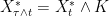We now prove that solutions to (3) for ${c\le1}$ are proper martingales. It is sufficient to show that its maximum process ${X^*_t}$ is square integrable, as it would follow that it is a local martingale of class (DL), which is equivalent to the martingale property. Letting ${\tau}$ be the first time at which X hits a value ${K>x}$ then ${X^*_{\tau\wedge t}=X^*_t\wedge K}$ is bounded and, in particular, is square integrable. Applying the quadratic version of the Burkholder-Davis-Gundy inequality gives

$\displaystyle {\mathbb E}[(X^*_{\tau\wedge t})^2]\le{\mathbb E}[X_0^2]+4{\mathbb E}[[X]_t]=x^2+4\int_0^t{\mathbb E}[1_{\{s\le\tau\}}X_s^{2c}]\,ds.$

As we are assuming that ${c\le1}$ , the inequality ${x^{2c}\le1+x^2}$ holds, giving

$\displaystyle {\mathbb E}[(X_t^*\wedge K)^2]\le x^2+4\int_0^t(1+{\mathbb E}[(X^*_s\wedge K)^2])\,ds.$

Applying Gronwall’s inequality to this gives the bound ${{\mathbb E}[(X^*_t\wedge K)^2]\le e^{4t}(x^2+1)-1}$ and, letting K increase to infinity, monotone convergence shows that ${{\mathbb E}[(X^*_t)^2]}$ satisfies the same bound. So, ${X^*_t}$ is square-integrable as required. Note that this argument works whenever the coefficients of the stochastic differential equation grow no faster than linearly in X.

To describe the further properties of X, we transform it into a squared Bessel process. Recall that applying the scale function to a Bessel process leads to a solution to (3). Let Z be a nonnegative solution to

$\displaystyle dZ_t=2\sqrt{Z_t}\,dW_t + 1_{\{Z_t>0\}}n\,dt$

(10)

for a Brownian motion W and, if Z hits zero then we assume that it sticks there. For real ${n\ge0}$ , this is a squared Bessel process of dimension n stopped when it hits zero. Assuming that ${n\not=2}$ , define the constants

$\displaystyle b=1-\frac{n}{2},\ a=(2b)^{-2}, c=1-\frac{1}{2b}=\frac{1-n}{2-n}$

(11)

and make the substitution ${X=(aZ)^b}$ . An application of Ito’s lemma shows that X does indeed solve (3) with ${B=W}$ (if ${n<2}$ ) or ${B=-W}$ (if ${n>2}$ ). Conversely, if X is a solution to (3) then ${Z=a^{-1}X^{1/b}}$ solves (10). Note that, in (11), ${c<1}$ and ${c>1}$ correspond to ${n<2}$ and ${n>2}$ respectively.

Let us apply this transformation, starting with the case ${c<1}$ or, equivalently, ${n<2}$ . If ${0\le n<2}$ then Z is a ${{\rm BES}^2_n}$ process stopped when it hits zero. Such Bessel processes always hit zero with probability one. For negative n, the process Z is not, strictly speaking, a Bessel process. It should still be clear that in this case, it has negative drift and must hit zero. In fact, both Z and ${M_t=Z_t-n\int_0^t1_{\{Z_s>0\}}\,ds}$ are nonnegative local martingales, so must converge to a finite limit. Therefore, ${\int_0^\infty1_{\{Z_s>0\}}\,ds}$ is almost-surely finite, and Z hits zero in a finite time. In any case, this shows that Z and, hence, ${X=(aZ)^b}$ almost surely hit zero.

For the remainder of this post, we consider the case with ${c>1}$ . Then, ${n>2}$ , ${b<0}$ , Z is a ${{\rm BES}^2_n}$ process and, therefore, ${X=(aZ)^b}$ can never hit zero. We look at the expected values of ${X^p}$ for a fixed positive p. Writing these in terms of Z,

$\displaystyle {\mathbb E}[X_t^p]=a^{-r}{\mathbb E}[Z_t^{-r}],$

for ${r=-bp\ge0}$ . We start by finding a simple upper bound. By properties of sums of independent Bessel processes, we can write ${Z=U+V}$ where U and V are independent squared Bessel processes of dimension n and 0 respectively, and with ${U_0=0}$ . Then, ${U_t/t}$ is a ${\chi^2_n}$ -distributed random variable, with probability density function

$\displaystyle p_n(u)=\frac{1}{2^{n/2}\Gamma(\frac n2)}u^{n/2-1}e^{-u/2},$

where ${\Gamma}$ is the gamma function. Then,

$\displaystyle \setlength\arraycolsep{2pt} \begin{array}{rl} {\mathbb E}[Z_t^{-r}]&\displaystyle\le t^{-r}{\mathbb E}[(U_t/t)^{-r}]\smallskip\\ &\displaystyle= \frac{t^{-r}}{2^{n/2}\Gamma(\frac n2)}\int_0^\infty u^{-r+n/2-1}e^{-u/2}\,du\smallskip\\ &\displaystyle=\frac{\Gamma(\frac n2-r)}{\Gamma(\frac n2)}(2t)^{-r}. \end{array}$

(12)

The integral above is only finite if ${r<n/2}$ or, equivalently, ${p<2c-1}$ , which we assume is the case. Then, as claimed, ${{\mathbb E}[X_t^p]}$ vanishes as time goes to infinity.

Before moving on, it is interesting to to note that the bound (12) does not depend at all on the initial value of Z. Also, as previously noted, the fact that X vanishes at infinity in the ${L^p}$ norm means that cannot be a martingale. It is possible to use this together with the (homogeneous) Markov property to show that the strict inequality (4) holds. However, we can also calculate a precise expression for ${{\mathbb E}[X_t^p]}$ , from which (4) will follow, which we now do.

Letting ${y=x^{1/b}/a}$ be the initial value of Z, then ${Z_t/t}$ has the ${\chi^2_n(y/t)}$ distribution. This can be constructed as follows: Let N be Poisson with parameter ${y/(2t)}$ and then, conditional on N, suppose that ${Z_t/t\sim\chi^2_{n+2N}}$ . This gives the correct distribution so, conditioning on N, the moments can be calculated in the same way as above

$\displaystyle {\mathbb E}[Z_t^{-r}\mid N]=\frac{\Gamma(\frac n2+N-r)}{\Gamma(\frac n2+N)}(2t)^{-r}.$

Taking the expected value of this, and substituting in ${v=y/(2t)}$ ,

$\displaystyle {\mathbb E}[Z_t^{-r}]=y^{-r}e^{-v}\sum_{k=0}^\infty\frac{\Gamma(\frac n2+k-r)}{k!\Gamma(\frac n2+k)}v^{k+r}.$

To decide whether this is increasing or decreasing in time, try differentiating with respect to v,

$\displaystyle \frac{d}{dv}{\mathbb E}[Z_t^{-r}]=y^{-r}e^{-v}\sum_{k=0}^\infty\frac{\Gamma(\frac n2+k-r)}{k!\Gamma(\frac n2+k)}\left((k+r)v^{k+r-1}-v^{k+r}\right).$

The terms in the summation can be reordered,

$\displaystyle \setlength\arraycolsep{2pt} \begin{array}{rl} &\displaystyle\frac{d}{dv}{\mathbb E}[Z_t^{-r}]=ry^{-r}e^{-v}\frac{\Gamma(\frac n2-r)}{\Gamma(\frac n2)}v^{r-1}\smallskip\\ &\displaystyle+y^{-r}e^{-v}\sum_{k=0}^{\infty}\left(\frac{\Gamma(\frac n2+k+1-r)}{(k+1)!\Gamma(\frac n2+k+1)}(k+r+1)-\frac{\Gamma(\frac n2+k-r)}{k!\Gamma(\frac n2+k)}\right)v^{k+r} \end{array}$

Applying the identities ${\Gamma(s+1)=\Gamma(s)s}$ and ${(k+1)!=k!(k+1)}$ and rearranging gives,

$\displaystyle \setlength\arraycolsep{2pt} \begin{array}{rl} \displaystyle\frac{d}{dv}{\mathbb E}[Z_t^{-r}]&\displaystyle=ry^{-r}e^{-v}\frac{\Gamma(\frac n2-r)}{\Gamma(\frac n2)}v^{r-1}\smallskip\\ &\displaystyle+ry^{-r}e^{-v}\left(\frac n2-r-1\right)\sum_{k=0}^\infty\frac{\Gamma(\frac n2+k-r)}{(k+1)!\Gamma(\frac n2 +k+1)}v^{k+r}. \end{array}$

(13)

If ${n/2-r-1\ge0}$ or, equivalently, ${p\le1}$ , then (13) is positive and ${{\mathbb E}[Z_t^{-r}]}$ is a strictly increasing function of v. So, ${{\mathbb E}[X_t^p]=a^{-r}{\mathbb E}[Z_t^{-r}]}$ is a strictly decreasing function of time, and is bounded. If, on the other hand, ${p\ge1}$ , the last term in (13) is negative. Integrating gives the inequality

$\displaystyle {\mathbb E}[Z_t^{-r}]\le ry^{-r}\frac{\Gamma(\frac n2-r)}{\Gamma(\frac n2)}\int_0^{y/(2t)}v^{r-1}e^{-v}\,dv.$

Substituting X back in gives the following bound

$\displaystyle \setlength\arraycolsep{2pt} \begin{array}{rl} \displaystyle{\mathbb E}[X_t^p]&\displaystyle\le rx^p\frac{\Gamma(\frac n2-r)}{\Gamma(\frac n2)}\int_0^{y/(2t)}v^{r-1}e^{-v}\,dv\smallskip\\ &\displaystyle<rx^p\frac{\Gamma(\frac n2-r)}{\Gamma(\frac n2)}\Gamma(r). \end{array}$

So, X is ${L^p}$ -bounded as promised. Finally, fix a time s and apply the above argument to the time-shifted process ${\tilde X_t\equiv X_{s+t}}$ to get,

$\displaystyle {\mathbb E}[X_t^p\mid\mathcal{F}_s]<rX_s^p\frac{\Gamma(\frac n2-r)}{\Gamma(\frac n2)}\Gamma(r)$

(almost surely) for all ${t>s}$ . Putting p=1 and r=n/2-1 into this gives ${{\mathbb E}[X_t\mid\mathcal{F}_s]<X_s}$ .

5 thoughts on “Failure of the Martingale Property”

Nils Framstad says:

16 August 10 at 7:12 PM

A couple of comments:

1) In finance, it is not uncommon to exclude doubling strategies by imposing an L^2 property (for convenience — a more natural modeling choice is to impose a lower bound on intermediate market value), which is effectively the restriction of the integral to the basic square-integrable case where the isometry holds. For this reason, practitioners may choose to define the integral only on L^2. So in order to discuss whether an integral wrt. Brownian motion fails to be a martingale, one should be cautious to specify the domain of the Ito integral.

2) How often have one seen CEV models just stated without any thought on whether (i) they may hit 0, or (ii) if 0 is reflecting or absorbing? So old news it is frequently forgotten.

A few references for the interested reader:
D. C. Emanuel and J. D. MacBeth in J. of Financial and Quantitative Analysis (1982) on the failure of the martingale property in the CEV context
R. Dudley in A.A.P. (open access), outside the diff.eq. setting, but hey, a striking page-and-a-half paper.
Y. Kabanov points out that the situation is different in discrete time: http://ideas.repec.org/a/spr/finsto/v12y2008i3p293-297.html (non-open).

1. George Lowther says:
  
  16 August 10 at 11:50 PM
  
  Thanks for those comments and references.
  
  The following use of the strict local martingale property to option pricing also looks interesting: Local martingales, bubbles and option prices, by Alexander M. G. Cox and David G. Hobson (Finance and Stochastics, 2005). They give several examples of strict local martingales, including the CEV case, point out that this does not introduce arbitrage as long as you restrict to admissible strategies (which necessarily cannot include short selling a fixed quantity over a fixed time period), and describe several ways in which option pricing deviates from the martingale case.
  
kenneth says:

6 June 13 at 3:50 PM

Following equation (11), you claimed $X = (a Z)^b$ solves (3) with $B = -W$ for $n>2$. But, my calculation leads to such $X$ solves (3) with $B = W$ even for $n>2$. For instance, when $n = 3$, we have $d X = Z^{-1} d W = X^2 dW$. Am I missing some trivial facts? Thanks.

kenneth says:

6 June 13 at 4:09 PM

@George, Sorry it’s my calculation mistake. I forgot that the sign of a is always positive.

Pingback: Strictly local martingales: what is the intuition behind them? | DL-UAT

	Anonymous on About
	Anonymous on About
	Anonymous on The Stochastic Integral
	Anonymous on Bessel Processes
	Anonymous on Bessel Processes
	Stat Prof on Pathwise Regularity of Optiona…
	Yang Chu on Spitzer’s Formula
	Anonymous on About
	Anonymous on Continuous Processes with Inde…
	Anonymous on Continuous Processes with Inde…

Failure of the Martingale Property

The Martingale Property in Option Pricing

Properties of the SDE

Published by George Lowther

5 thoughts on “Failure of the Martingale Property”

Leave a comment Cancel reply

The Martingale Property in Option Pricing

Properties of the SDE

Related

Published by George Lowther

5 thoughts on “Failure of the Martingale Property”

Leave a comment Cancel reply