Martingales are Integrators

A major foundational result in stochastic calculus is that integration can be performed with respect to any local martingale. In these notes, a semimartingale was defined to be a cadlag adapted process with respect to which a stochastic integral exists satisfying some simple desired properties. Namely, the integral must agree with the explicit formula for elementary integrands and satisfy bounded convergence in probability. Then, the existence of integrals with respect to local martingales can be stated as follows.

Theorem 1 Every local martingale is a semimartingale.

This result can be combined directly with the fact that FV processes are semimartingales.

Corollary 2 Every process of the form X=M+V for a local martingale M and FV process V is a semimartingale.

Working from the classical definition of semimartingales as sums of local martingales and FV processes, the statements of Theorem 1 and Corollary 2 would be tautologies. Then, the aim of this post is to show that stochastic integration is well defined for all classical semimartingales. Put in another way, Corollary 2 is equivalent to the statement that classical semimartingales satisfy the semimartingale definition used in these notes. The converse statement will be proven in a later post on the Bichteler-Dellacherie theorem, so the two semimartingale definitions do indeed agree.

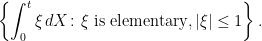
Let us now move on to the proof of Theorem 1 noting that, by localization, it is sufficient to prove the result for proper martingales. The previous post on existence of stochastic integrals will be used. To show that a cadlag martingale X is a semimartingale, we need to prove that the following set of elementary integrals is bounded in probability for each positive time t.

$\displaystyle \left\{\int_0^t\xi\,dX\colon \xi\textrm{ is elementary}, \vert\xi\vert\le 1\right\}.$

This is equivalent to stating that there is a function ${f\colon{\mathbb R}_+\rightarrow{\mathbb R}_+}$ such that f(K) tends to zero as K goes to infinity and,

$\displaystyle {\mathbb P}\left(\left\vert\int_0^t\xi\,dX\right\vert> K\right)\le f(K)$

(1)

for all elementary predictable ${\vert\xi\vert\le 1}$ . As always in these notes, we work with respect to a complete filtered probability space ${(\Omega,\mathcal{F},\{\mathcal{F}_t\}_{t\ge 0},{\mathbb P})}$ . Then, on any interval (0,t], an elementary process ${\xi}$ can be written in the form

$\displaystyle 1_{\{0<s\le t\}}\xi_s=\sum_{k=1}^nZ_k1_{\{t_{k-1}<s\le t_k\}}$

(2)

for times ${0=t_0<t_1<\cdots<t_n=t}$ and ${\mathcal{F}_{t_{k-1}}}$ -measurable random variables ${Z_k}$ . For such integrands, the stochastic integral is

$\displaystyle \int_0^t \xi\,dX = \sum_{k=1}^n Z_k(X_{t_k}-X_{t_{k-1}}).$

(3)

The proof that X is is semimartingale is easiest for square integrable martingales, so we handle that case first before generalizing to arbitrary martingales.

Square Integrable Martingales

The aim for now is to prove the following result for square integrable martingales.

Lemma 3 Let X be a square integrable martingale and ${\vert\xi\vert\le 1}$ be elementary predictable. Then,

$\displaystyle {\mathbb E}\left[\left(\int_0^t\xi\,dX\right)^2\right]\le{\mathbb E}[X_t^2]-{\mathbb E}[X_0^2].$ (4)

Then, by Chebyshev’s inequality, (1) will hold for ${f(K)=K^{-2}{\mathbb E}\left[ X_t^2\right]}$ so, once the above lemma is established it will follow that all cadlag square integrable martingales are indeed semimartingales.

For the remainder of this section, assume that ${\xi}$ is as in (2). Restricting to the finite set of times ${t_k}$ gives the discrete filtration ${\{\mathcal{F}_{t_k}\}_{k=0,1,\ldots,n}}$ , reducing the problem to one involving only discrete-time stochastic processes. Given a discrete-time process ${\{Y_k\}_{k=0,1,\ldots,n}}$ denote its increments ${\delta Y}$ , quadratic variation [Y] and `integral’ ${Z\cdot Y}$ (for a discrete-time integrand Z) as follows,

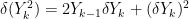
$\displaystyle \setlength\arraycolsep{2pt} \begin{array}{rl} \displaystyle\delta Y_k&\displaystyle\equiv Y_k-Y_{k-1},\smallskip\\ \displaystyle Z\cdot Y_k&\displaystyle\equiv\sum_{j=1}^k Z_j\delta Y_j,\smallskip\\ \displaystyle [Y]_k &\displaystyle\equiv \sum_{j=1}^k(\delta Y_j)^2. \end{array}$

The identity ${[Z\cdot Y]=Z^2\cdot[Y]}$ follows immediately from this. Summing ${\delta (Y^2_k)=2Y_{k-1}\delta Y_k+(\delta Y_k)^2}$ over k gives the following discrete integration by parts formula

$\displaystyle Y^2 = Y_0^2 + 2Y_{-}\cdot Y + [Y],$

(5)

where ${Y_-}$ denotes the process ${1_{\{k>0\}}Y_{k-1}}$ . If, furthermore, Y is a discrete square integrable martingale, so that ${{\mathbb E}[\delta Y_k\mid\mathcal{F}_{t_{k-1}}]=0}$ , then taking expectations gives

$\displaystyle {\mathbb E}[Y^2] = {\mathbb E}\left[Y_0^2+[Y]\right].$

(6)

Note also that if Y is a martingale and Z is a bounded and `discrete predictable’ process (i.e, ${Z_k}$ is ${\mathcal{F}_{t_{k-1}}}$ -measurable), then ${{\mathbb E}[\delta(Z\cdot Y_k)\mid\mathcal{F}_{t_{k-1}}]=Z_k{\mathbb E}[\delta Y_k\mid\mathcal{F}_{t_{k-1}}]=0}$ . So, ${Z\cdot Y}$ will also be a martingale, and can be used in the place of Y in (6) to obtain the discrete version of Ito’s isometry,

$\displaystyle {\mathbb E}[(Z\cdot Y)^2] = {\mathbb E}\left[Z^2\cdot[Y]\right],$

which holds for square integrable martingales Y and bounded predictable Z. Finally, if ${\vert Z\vert\le 1}$ then Ito’s isometry gives the inequality

$\displaystyle {\mathbb E}[(Z\cdot Y)^2] \le{\mathbb E}\left[[Y]\right]={\mathbb E}[Y^2]-{\mathbb E}[Y_0^2].$

(7)

So, setting ${Y_k=X_{t_k}}$ and letting Z be as in (2), equation (3) can be written as ${\int_0^t\xi\,dX=Z\cdot Y_n}$ . So, (7) gives inequality (4) as required.

General Martingales

Lemma 4 There exists a constant c such that the following inequality holds for any martingale X, elementary ${\vert\xi\vert\le 1}$ and positive real number K.

$\displaystyle {\mathbb P}\left(\left\vert\int_0^t\xi\,dX\right\vert\ge K\right)\le \frac{c}{K}{\mathbb E}\vert X_t\vert.$ (8)

Taking ${f(K)=cK^{-1}{\mathbb E}\vert X_t\vert}$ in (1), this result shows that cadlag martingales are indeed semimartingales. It was shown by Burkholder that the optimal value for c is 2 (Sharp norm comparison of martingale maximal functions and stochastic integrals). However, for the purposes of proving Theorem 1 it is only necessary to prove the result for some c, and we do not attempt to find the best value.

The idea behind the proof of the lemma is to stop the martingale X before it gets too large, and then the previous method for square integrable martingales can be applied. It helps to first choose any time ${t_{n+1}>t}$ . Then, define the stopping time

$\displaystyle \tau=\min\left\{t_k\colon k=0,1,\ldots,n,\ \vert X_{t_k}\vert\ge K\right\}\cup\{t_{n+1}\}.$

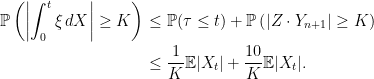
Doob’s inequality bounds the probability that the maximum of X exceeds K,

$\displaystyle {\mathbb P}\left(\max_{k\le n}\vert X_{t_k}\vert \ge K\right)={\mathbb P}(\tau\le t)\le\frac{1}{K}{\mathbb E}\vert X_t\vert.$

Next, define the discrete process Y to be equal to X prior to ${\tau}$ and 0 afterwards

$\displaystyle Y_k = 1_{\{t_k<\tau\}} X_{t_k}.$

By definition, this is uniformly bounded by K and ${Y_{n+1}=0}$ . Also, letting Z be as in (2) and taking ${Z_{n+1}=0}$ gives

$\displaystyle Z\cdot Y_n=Z\cdot Y_{n+1}=\int_0^t\xi\,dX$

(9)

whenever ${\tau> t}$ . Unfortunately, the process Y is not a martingale. However, it can be approximated by the stopped process ${\tilde Y_k=X_{t_k\wedge t\wedge\tau}}$ , which satisfies ${\delta \tilde Y_k-\delta Y_k=1_{\{t_k=\tau\}}X_{\tau\wedge t}}$ . Also, by the martingale property, ${{\mathbb E}[H\cdot\tilde Y]=0}$ for any discrete, predictable and bounded process H. If, furthermore, ${\vert H\vert\le 1}$ then, letting m be such that ${t_m=\tau}$ ,

$\displaystyle \setlength\arraycolsep{2pt} \begin{array}{rl} \displaystyle{\mathbb E}[H\cdot Y_k]&\displaystyle={\mathbb E}[H\cdot (Y-\tilde Y)_k]\smallskip\\ &\displaystyle=-{\mathbb E}[1_{\{t_k\ge\tau>0\}}H_mX_{\tau\wedge t}]\smallskip\\ &\displaystyle=-{\mathbb E}[1_{\{t_k\ge\tau> 0\}}H_mX_t]\smallskip\\ &\displaystyle\le{\mathbb E}\vert X_t\vert. \end{array}$

(10)

Now, a Doob decomposition ${Y=Y_0+M+A}$ is used, where M is a discrete martingale and A is a discrete predictable process, both starting at 0. The processes M and A are defined by

$\displaystyle \delta A_k = {\mathbb E}[\delta Y_k\mid\mathcal{F}_{t_{k-1}}],\ \delta M_k = \delta Y_k-\delta A_k.$

The following identity follows from this definition,

$\displaystyle {\mathbb E}[(\delta Y_k)^2\mid\mathcal{F}_{t_{k-1}}]={\mathbb E}[(\delta M_k)^2\mid\mathcal{F}_{t_{k-1}}]+(\delta A_k)^2$

Taking expectations and summing over k,

$\displaystyle {\mathbb E}\left[ [Y]\right] = {\mathbb E}\left[ [M]+[A] \right]\ge{\mathbb E}\left[ [M]\right].$

Then applying (7) gives the following bound for the integral with respect to M,

$\displaystyle \setlength\arraycolsep{2pt} \begin{array}{rl} \displaystyle{\mathbb E}\left[(Z\cdot M_{n+1})^2\right] &\displaystyle\le {\mathbb E}\left[ [M]_{n+1}\right]\le{\mathbb E}\left[[Y]_{n+1}\right]\smallskip\\ &\displaystyle={\mathbb E}[Y_{n+1}^2-Y_0^2-2Y_-\cdot Y_{n+1}]\smallskip\\ &\displaystyle\le -2{\mathbb E}[Y_-\cdot Y_{n+1}]\smallskip\\ &\displaystyle\le 2K{\mathbb E}\vert X_t\vert. \end{array}$

This makes use of the integration by parts formula (5) and, as ${Y_{n+1}=0}$ , the inequality ${Y^2_{n+1}-Y^2_0\le 0}$ is used. The final inequality comes from (10) with ${-K^{-1}Y_-}$ in place of H. So, Chebyshev’s inequality can be used to bound the probability

$\displaystyle {\mathbb P}\left(\vert Z\cdot M_{n+1}\vert\ge K/2\right)\le \frac{4}{K^2}{\mathbb E}[(Z\cdot M_{n+1})^2]\le\frac{8}{K}{\mathbb E}\vert X_t\vert.$

(11)

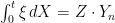
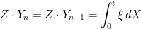
Let us now look at the integral with respect to A. Defining ${\tilde Z_k={\rm sgn}(Z_k\delta A_k)Z_k}$ gives ${\tilde Z_k\delta A_k=\vert Z_k\delta A_k\vert}$ and the following is obtained,

$\displaystyle {\mathbb E}\left[\vert Z\cdot A\vert\right]\le{\mathbb E}[\tilde Z\cdot A] = {\mathbb E}[ \tilde Z\cdot Y]\le{\mathbb E}\vert X_t\vert,$

using (10) for the final inequality. So, applying Chebyshev’s inequality one more time,

$\displaystyle {\mathbb P}\left(\vert Z\cdot A\vert\ge K/2\right)\le\frac{2}{K}{\mathbb E}\left[\vert Z\cdot A\vert\right]\le\frac{2}{K}{\mathbb E}\vert X_t\vert.$

Combining this with (11) ,

$\displaystyle \setlength\arraycolsep{2pt} \begin{array}{rl} \displaystyle{\mathbb P}\left(\vert Z\cdot Y_{n+1}\vert\ge K\right) &\displaystyle\le{\mathbb P}\left(\vert Z\cdot M_{n+1}\vert\ge K/2\right) +{\mathbb P}\left(\vert Z\cdot A_{n+1}\vert\ge K/2\right)\smallskip\\ &\displaystyle\le \frac{10}{K}{\mathbb E}\vert X_t\vert. \end{array}$

Finally, using expression (9) for the integral when ${\tau>t}$ gives (8) as required,

$\displaystyle \setlength\arraycolsep{2pt} \begin{array}{rl} \displaystyle{\mathbb P}\left(\left\vert\int_0^t\xi\,dX\right\vert\ge K\right) &\displaystyle\le\displaystyle{\mathbb P}(\tau\le t) + {\mathbb P}\left(\vert Z\cdot Y_{n+1}\vert\ge K\right)\smallskip\\ &\displaystyle\le\frac{1}{K}{\mathbb E}\vert X_t\vert+\frac{10}{K}{\mathbb E}\vert X_t\vert. \end{array}$

Notes

It is also possible to construct the integral with respect to any cadlag martingale without relying on the previous post on existence of stochastic integrals. This isn’t any less work than the proof used above though.

First, for a square integrable and cadlag martingale X, define the linear function ${DX^2}$ on the space of bounded elementary processes,

$\displaystyle DX^2(\xi) \equiv{\mathbb E}\left[\int_0^\infty\xi\,d(X^2)\right].$

As ${X^2}$ is a submartingale, this is a positive map. The following identity is straightforward,

$\displaystyle {\mathbb E}\left[\left(\int_0^t\xi\,dX\right)^2\right]=DX^2(1_{(0,t]}\xi^2).$

(12)

Furthermore, using the fact that positive submartingales are of class (DL), it can be shown that ${DX^2}$ is countably additive on the nonnegative elementary processes. Then, Carathéodory’s extension theorem allows ${DX^2}$ to be extended to a measure on ${({\mathbb R}_+\times\Omega,\mathcal{P})}$ , which is known as the Doléans measure of ${X^2}$ . So, for each positive time t, ${\langle\alpha,\beta\rangle\equiv DX^2(1_{(0,t]}\alpha\beta)}$ defines an inner product on the space of bounded predictable processes and equation (12) says that the stochastic integral is an isometry from the elementary processes to ${L^2(\Omega,\mathcal{F},{\mathbb P})}$ . It can then be uniquely extended as an isometry from the space of bounded predictable processes.

The extension to an arbitrary cadlag martingale X can be achieved by approximating by a sequence ${X^n}$ of square integrable martingales, so that ${{\mathbb E}\vert X^n_t-X_t\vert\rightarrow 0}$ . Lemma 4 implies that convergence also holds under the semimartingale topology so that, by completeness, X will also be a semimartingale.

Compare this approach to the classical proof, which uses the Ito isometry for square integrable martingales

$\displaystyle {\mathbb E}\left[\left(\int_0^t\xi\,dX\right)^2\right] = {\mathbb E}\left[\int_0^t\xi^2\,d\langle X\rangle\right],$

where ${\langle X\rangle}$ is an increasing process such that ${X^2-\langle X\rangle}$ is a martingale. The extension to arbitrary local martingales involves a decomposition X=M+V, for a locally square integrable martingale M and FV process V. The method outlined here with the Doléans measure avoids the rather involved construction of ${\langle X\rangle}$ and decompositions of martingales. The proof given in the main body of this post also avoids having to construct the Doléans measure, instead relying on a characterization of semimartingales in terms of boundedness in probability.

4 thoughts on “Martingales are Integrators”

Anonymous says:

20 January 21 at 11:59 AM

Dear George,

I wonder, why we need the extra work after we prove that every square integrable martingale is a semimartingale. Isn’t true that every martingale is locally bounded, so locally square integrable ?

1. George Lowther says:
  
  20 January 21 at 8:30 PM
  
  Not every martingale is locally square integrable. If its jumps are not locally square integrable, then the process won’t be either.
  
  1. Anonymous says:
    
    21 January 21 at 12:30 PM
    
    Dear George,
    
    Yes I see, however a proof along those lines I believe is possible if we also stop the prosses $(\Delta X)^*$ . But, I suppose we can’t avoid the use of the projection theorem that way, although the proof in your notes for this result is elementary.
    
    1. George Lowther says:
      
      21 January 21 at 4:52 PM
      
      Yes, you can build a proof along those lines. Stop the martingale when it hits some level. The stopped process may not be locally square integrable. However, if you subtract out the jump at that time, and add back the compensator of the jump, you will get a locally bounded martingale. Then you need to add back the jump minus its compensator (which is of finite variation). However, that involves more continuous time stochastic process theory than I wanted to use here.
      
      Edit: In fact, the proof in this post is along similar lines to the continuous time approach just mentioned. The difference is that I effectively prove it in discrete time, but give a quantitative result, so that the continuous time result also holds with the same quantitative bound.

	Anonymous on About
	Anonymous on About
	Anonymous on The Stochastic Integral
	Anonymous on Bessel Processes
	Anonymous on Bessel Processes
	Stat Prof on Pathwise Regularity of Optiona…
	Yang Chu on Spitzer’s Formula
	Anonymous on About
	Anonymous on Continuous Processes with Inde…
	Anonymous on Continuous Processes with Inde…